Brief Introduction to Gradient Descent

Brief Introduction to Gradient Descent.

This blog gives a brief overview of the Gradient descent optimization algorithm which is highly used in machine learning and deep learning. Gradient descent is used by many machine learning practioner's including myself.

Everyday we use optimization techniques and algorithms with or without knowledge. For example for getting a shorter path between two paths we prefer shorter path rather the longest path which takes more time. Optimization is at the heart of most of the statistical and Machine Learning techniques which are widely used in data science. for example, you may use a gradient descent algorithm to optimize the parameters used in the machine learning model which gives accurate results.

What is Gradient Descent in Machine Learning?

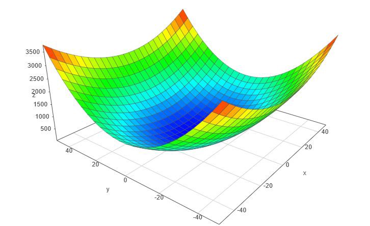
Gradient Descent is an iterative process that finds the minima of a function. Gradient descent is an optimization algorithm mainly used to find the minimum of a function. In machine learning, gradient descent is used to update parameters in a model. Parameters can vary according to the algorithms, such as coefficients in Linear Regression and weights in Neural Networks.
Let’s take an example of a Simple Linear regression problem where our aim is to predict the dependent variable(y) when only one independent variable is given. for the above linear regression model, the equation of the line would be as follows.
y = m x + c
Our ultimate goal of the optimization algorithm is to minimize the loss function. Let's take MSE(mean sqaured error) loss function which actually computes the loss given by the current parameters of the model.

In the above equation,
• y is the dependent variable
• x is the independent variable
• m is the slope of the line
• c is the intercept on the y-axis by the line
Our ultimate goal of the optimization algorithm is to minimize the loss function. Let's take MSE(mean sqaured error) loss function which actually computes the loss given by the current parameters of the model.

Loss Function

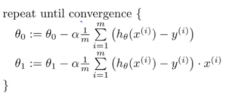
Here we are required to optimize the value of ‘m’ and ‘c’ in order to minimize the Loss function. as y_predicted is the output given by the Linear Regression Equation, therefore Loss at any given point can be given by In order to find out the negative of the slope, we proceed by finding the partial derivatives with respect to both ‘m’ and ‘c’ partial derivatives w.r.t m and c When 2 or more than 2 partial derivatives are done on the same equation w.r.t to 2 or more than 2 different variables, it is known as Gradient. After performing partial derivatives w.r.t to ‘m’ and ‘c’ we obtain 2 equations as given above; when some value of ‘m’ and ‘c’ is given and is summed across all the data points, we obtain the negative side of the slope. The next step is to assume a Learning Rate, which is generally denoted by ‘α’ (alpha). In most cases, the Learning Rate is set very close to 0 e.g., 0.001 or 0.005. A small learning rate will result in too many steps by the gradient descent algorithm and if a large value of ‘α’ is selected, it may result in the model to never converging at the minima. Next is to determine Step Size based on our Learning Rate. Step Size can be defined as finding the next points using the learning rate This will give us 2 points which will represent the updated value of ‘m’ and ‘c’. We Iterate over the steps of finding the negative of the slope and then update the value of ‘m’ and ‘c’ until we reach or converge on our minima.

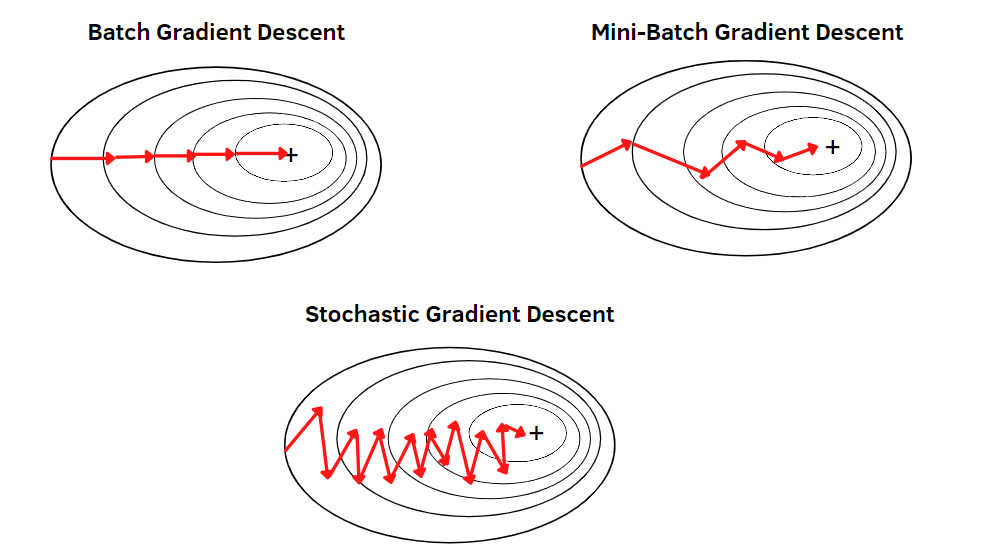
Types of gradient descent

1) Batch gradient descent
In this type of gradient descent, all the training examples are processed for each iteration of gradient descent. It gets computationally expensive if the number of training examples is large. This is when batch gradient descent is not preferred. Rather a stochastic gradient descent or mini-batch gradient descent is used.

2) Stochastic gradient descent
The word stochastic is related to a system or process linked with a random probability. Therefore, in Stochastic Gradient Descent (SGD), samples are selected at random for each iteration instead of selecting the entire data set. When the number of training examples is too large, it becomes computationally expensive to use batch gradient descent. However, Stochastic Gradient Descent uses only a single sample, i.e., a batch size of one, to perform each iteration. The sample is randomly shuffled and selected for performing the iteration. The parameters are updated even after one iteration, where only one has been processed. Thus, it gets faster than batch gradient descent.

3) Mini-batch gradient descent
This type of gradient descent is faster than both batch gradient descent and stochastic gradient descent. Even if the number of training examples is large, it processes it in batches in one go. Also, the number of iterations is lesser despite working with larger training samples.

Challenges in Executing Gradient Descent

There are many cases where gradient descent fails to perform well. There are mainly three reasons why this would happen:
• Data challenges
• Gradient challenges
• Implementation challenges

Conclusion

This brings us to the end of this article, where we have learned about What is Gradient Descent in machine learning and how it works. Its various types of algorithms, challenges we face with gradient descent